In order to give you a feeling how to use AIM2000, we will explain the main features of the program by presenting an example. We decided for Tetrahedrane since it is a simple molecule with 14 molecular orbitals. The 4 carbon atoms form a tetrahedron and we expect to find all four kinds of critical points in the charge density.
After starting AIM2000, we load the wavefunction of Tetrahedrane into the program. Immediately you can see a display of the 8 atoms in 3D-View.

The first step of the AIM-analysis of a molecule is always the determination of critical points of the charge density (which is the default density function in Control View). Therefore we choose "critical points" from the calculation menu. Alternatively the corresponding button in the tool bar can be used.
The critical point dialog appears. The main difficulty in calculating critical points is the choice of starting values for Newton's method. AIM2000 supports you by providing some power methods (Starting iterations at ...):
... nuclear positions. This will find us all 8 charge density maxima ((3,-3) - critical points) which are always very close to nuclear positions.
... mean values of maxima pairs. After knowing the maxima, we expect to find (3, -1) - critical points between pairs of maxima and try for them. This method only gives us 6 of the 10 (3,-1) - critical points but all (3,+1) - critical points and the charge density minimum in the middle of the molecule. Note the list of nuclear positions and critical points on the right hand side of the dialog.
In order to find the missing critical points between carbon and hydrogen atoms, we could either try to guess better starting values or decrease the iteration stepsize. This forces Newton's method to stay longer in the region of the starting point.
Click "options" to open the critical point options dialog and change the stepsize factor for Newton iteration to 0.5. Try again "... mean values of maxima pairs" and you will find all critical points of the charge density in the list.


We now would like to have a look at some properties of one of the (3,-1) - critical points. Choose one from the list. Its coordinates appear in coordinate areas. Click "Analyse Starting Point" to open the "Properties of density functions" - dialog. Various properties of the chosen point are displayed.

A more complete set of information on this point can be optained by clicking "Write Data to Record View". After closing both dialogs, we find the data in the Record View and can (via file menu) display a Print Preview.

Close the Print Preview. Note the display of critical points in 3D-View.
Now we try to establish the molecular graph, i.e. those gradient paths which connect critical points. Choose "Molecular graph" from the caluclation menu. There are three kinds of molecular graph paths:
Bond paths connect (3,-1)-critical points with charge density maxima. Click on "Paths uphill from (3,-1) - critical points" and AIM2000 will quickly calculate all bond paths.
"Paths downhill from (3,+1) - critical points" are also easily computed. Each ring critical point has two, one of them terminating at the charge density minimum of C4H4.
There are also unique paths connecting (3,-1) with (3,+1) - critical points. Their calculation involves an iterative process since there is no unique direction for them on either side. The calculation for Tetrahedrane is pretty fast, but other molecule might present more problems ("Paths connecting (3,-1) and (3,+1) - critical points").
You can get short or long descriptions of selected paths by clicking the corresponding buttons at the bottom of the dialog.

After closing the molecular graph dialog, all computed paths are displayed in 3D-View (we got rid of the molecular coordinate axis via the context menu of 3D-View).

The whole structure analysis we did up to now for the charge density of Tetrahedrane can also be done for all other density functions. See the third list box in Control View.
We can now try to compute properties of the atoms in C4H4. Let's choose atom H5 in the first list box in Control View.
Choose "Integration over atomic basin" in the calculation menu. The integration dialog appears.
The integration process consists of two parts: First, integration is done in radial coordinates in a sphere around the nucleus which should totally be inside the atomic basin. The default radius of the sphere is 0.5. This is usually ok, only for Hydrogen atoms the sphere sometimes has to be smaller. We change the radius to 0.3.
In the list box on the right hand side all nuclei and critical points are listed with their atomic coordinates. This allows you to check their distance from our nucleus.
The other part of the integration uses natural coordinates outside the sphere.
By clicking "Integrate inside Beta-sphere" only the first part is performed, "Integrate in natural coordinates" performs both parts if necessary. We choose the latter.
After some time (for large wavefunctions time can be long!) the results are displayed.

Note the value for the Laplacian of Rho. It should be zero and gives you a feeling for the accuracy of the integration.
If the accuracy of these numbers is too low for your requirements, increase accuracies in the options dialog for basin integration (click "Options").
If you want to change the number of functions integrated, click "Functions". Select and deselect functions in the appearing dialog. For definitions of these functions, see AIM2000 user's guide.

We now integrate over the atomic basins of some other atoms: C1, C2, H6.
Note e.g. the results for C2:

After closing all dialogs and choosing C1 in the first list box of Control View, we can get a total record of this atom by choosing "atom" in the record menu.
Below you see the three pages of this print preview:


Now let us choose surface C1/H5 from the second list box in control View.
Similar to the basin integration we can calculate properties of this interatomic surface by integrating various functions.
Choose "Integration over interatomic surface" from the Calculation menu and click "Integrate" in the appearing dialog.
After a short time we can see the integration results.

Again, via the Record menu, we can get a record and a print preview of this interatomic surface.

Finally we want to produce some nice pictures, i.e. envelope maps.
First we have to do the lengthy calculation of a point grid covering the part of the molecule we are interested in.
From the Envelope menu choose "Initialize envelope grid".

We have various possibilities to save some work, but for now we take the defaults and compute a grid covering the whole molecule.
In order to get a better grid with smaller mesh size we choose "Increase grid density" from the Envelope menu three times! Each time the mesh size is halfed.
These calculations take some time since, for each point, the corresponding atomic basin has to be determined.
If you want to save your work in an .aim-file go ahead! But note that this .aim-file will contain all the grid data. It's size is about 60 MB.
We now open the envelope definition dialog: "Define envelope map" in the Envelope menu.
In order to get an impression of the charge density, we first produce an 0.1 au isosurface of Rho of the whole molecule.
For a nice picture we also choose a color (click Color buttons), set the transparency index to 0.2 and try for a triangularized view.

After switching on envelope maps in the context menu of 3D-View, the results looks like this:

Back into the envelope definition dialog. We now restrict our picture to the atoms C4 and H8, switch off transparency, and use spheres for display.

After clicking into 3D-View we get:

Again back into the envelope definition dialog, we restrict the picture to H8 and triangularize the envelope:

Of course we can also produce envelope maps of other density functions. For instance choose "L, Laplacian of Rho" from the third list box in Control View.
Open the envelope definition dialog and set the values according to the next screen shot:

We get a nice envelope map of the Laplacian:

If your computer is fast enough, you are able to rotate and zoom the picture with mouse and keyboard.
Now we can also generate some 2D plots for the documentation.


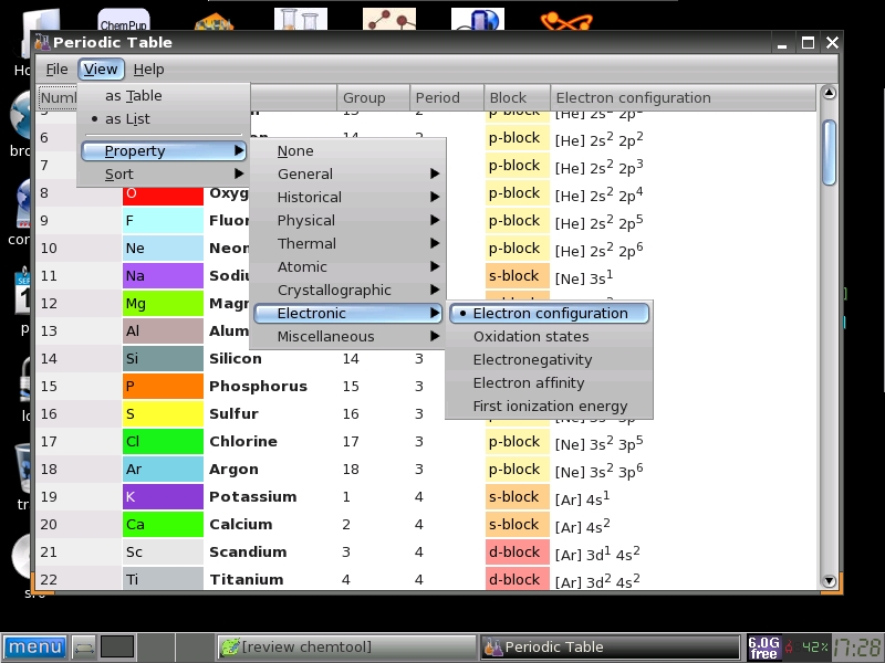
 Seperti
halnya aplikasi yang menyajikan tabel periodik, tentu akan memberikan
informasi sedatail mungkin dengan tampilan yang sangat menarik. Pada
GElement ini kita bisa melihat sifat-sifat terkait unsur masing-masing
mulai dari informasi yang tergolong umum, sifat fisik, maupun sifat
atomiknya.
Seperti
halnya aplikasi yang menyajikan tabel periodik, tentu akan memberikan
informasi sedatail mungkin dengan tampilan yang sangat menarik. Pada
GElement ini kita bisa melihat sifat-sifat terkait unsur masing-masing
mulai dari informasi yang tergolong umum, sifat fisik, maupun sifat
atomiknya.


 Aplikasi ini sangat cocok digunakan mengajarkan materi yang terkait sengan sistem periodik, struktur atom dan kimia unsur.


