KISI-KISI UTS KELAS XI IPA MAN 1 MAGELANG


1.       Bilangan kuantum
2.       Bilangan kuantum
3.       Menentukan jenis sub kulitdari orbital
4.       Set bilangan kuantum
5.       Menentukan banyaknya orbital
6.       Menentukan banyaknya orbital
7.       Menentukan bentuk molekul
8.       Bilangan kuantum
9.       Menentukan bentuk molekul
10.   Menentukan elektron valensi
11.   Menentukan senyawa polar
12.   Mengidentifikasi ikatan antar molekul
13.   Menentukan letak suatu unsur
14.   Menentukan letak suatu unsur
15.   Menentukan letak suatu unsur
16.   Menentukan jenis subkulit
17.   Menentukan letak suatu unsur
18.   Konfigurasi elektron ion
19.   Reaksi eksoterm dan endoterm
20.   Perubahan entalpi reaksi
21.   Reaksi eksoterm dan endoterm
22.   Reaksi eksoterm dan endoterm
23.   Reaksi eksoterm dan endoterm
24.   Perubahan entalpi reaksi
25.   Penentuan kalor reaksi
26.   Reaksi eksoterm dan endoterm
27.   Reaksi eksoterm dan endoterm
28.   Penentuan entalpi reaksi
29.   Reaksi eksoterm dan endoterm
30.   Penentuan kalor reaksi
31.   Persamaan termokimia
32.   Penentuan entalpi reaksi
33.   Penentuan entalpi reaksi
34.   Penentuan entalpi pembakaran
35.   Penentuan kalor reaksi
36.   Energi Ikatan
37.   Energi Ikatan
38.   Laju reaksi
39.   Laju reaksi
40.   Laju reaksi


ESSAY
1.       Meramalkan rumus dan bentuk molekul suatu senyawa
2.       Menuliskan set bilangan kuantum sub kulit
3.       Reaksi eksoterm dan endoterm
4.       Menghitung energi ikatan
5.       Penentuan perubahan entalpi reaksi netralisasi
 

GElement

GElement merupakan aplikasi yang dapat dipasang pada setiap sistem operasi Linux. 
Seperti halnya aplikasi yang menyajikan tabel periodik, tentu akan memberikan informasi sedatail mungkin dengan tampilan yang sangat menarik. Pada GElement ini kita bisa melihat sifat-sifat terkait unsur masing-masing mulai dari informasi yang tergolong umum, sifat fisik, maupun sifat atomiknya.
Dari tabel periodik ini kita juga bisa menelusuri lebih lanjut mengenai sumber yang dijadikan patokan pemberian nilai-nilai variabel sifat.
Berikut ini adalah screenshoot tampilan GElement model list (bukan dalam bentuk tabel seperti yang terlihat pada gambar-gambar sebelumnya). Kita bisa mengurutkan berdasarkan header table list yang ada juga bisa melihat sifat berdasarkan sifat umum (general), sejarah, sifat fisik, sifat termal, sifat atomik, bentuk kristalografik, elektronik dan sebagainya.

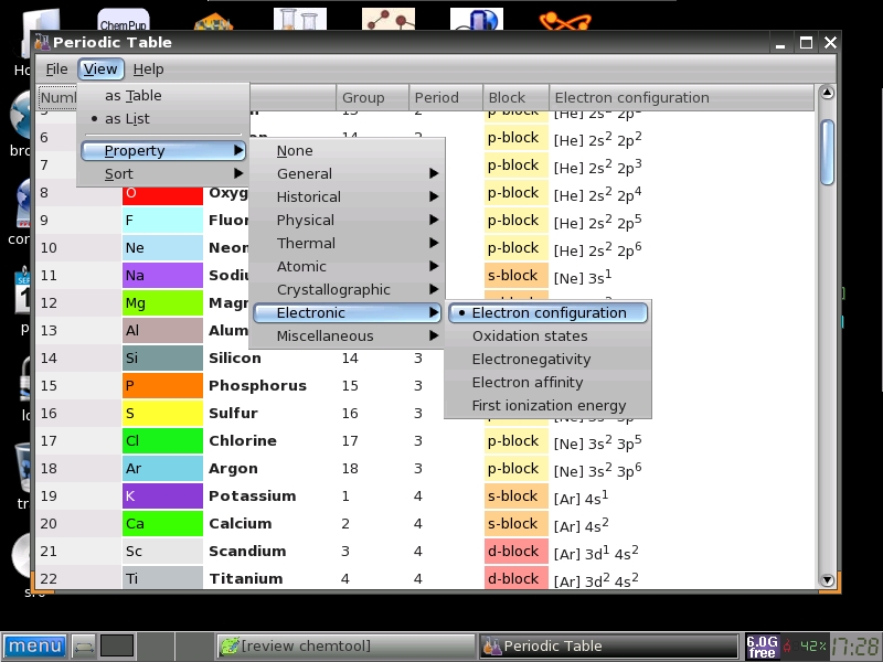
Aplikasi ini sangat cocok digunakan mengajarkan materi yang terkait sengan sistem periodik, struktur atom dan kimia unsur.

Molecule Viewer


 Molecule Viewer merupakan aplikasi kimia yang cukup simple karena fitur dalam aplikasi ini cukup sedikit. Kita dapat menggunakannya apabila kita telah menyimpan file molekul sebelumnya dan ingin melihat bentuk molekul yang telah kita simpan. Ada Ball and Sticks, Space Filling, Cylinders, dan Wireframe.
Saya memakai bentuk molekul H2SO4 yang sudah saya buat melalui aplikasi Avogadro.


Pengenalan Model Zig-zag dalam Menggambar Struktur Rantai Karbon


Bahasan senyawa karbon di buku-buku kimia sma selama ini masih belum banyak mengenalkan metode penulisan rantai karbon model zig-zag. Setahu saya pada buku kimia kelas 10 terbitan depdiknas (buku sekolah elektronik) hanya 1 buku dari 7 buku yang mengenalkan penulisan model zig-zag pada rantai karbon. Hanya dua buku yang menuliskan rumus struktur senyawa hidro karbon menggunakan software khusus untuk penggambaran rumus struktur kimia. Selebihnya menuliskannya secara manual menggunakan aplikasi olah kata. Bisa dibayangkan betapa melelahkannya melakukan cara manual seperti itu.

Selama ini struktur rantai karbon dikenalkan guru kimia ke siswa digambarkan dengan penggambaran model lurus saja. Jika begitu maka kewajiban menuliskan atom C pada penggambaran senyawa karbon. Tentu saja awalnya ini cukup sederhana dan mudah dipahami, namun sangat tidak efisien dalam penulisannya serta ini “jauh” dari struktur rantai karbon yang sesungguhnya.
Bagaimana kalau harus membuat presentasi dengan menggunakan aplikasi presentasi semacam ms. powerpoint, betapa sulitnya itu. Sama halnya kalau dalam bentuk teks seperti pada penulisan dalam berkas olah kata. Jelas itu menjadi sulit dan tidak praktis. Untuk membuat satu struktur sederhana dari metana saja harus diperlukan usaha ekstra.
Apakah guru kimia sekarang belum kenala dengan aplikasi menggambar rumus kimia atau rumus struktur? Mengapa tidak menggunakan aplikasi kimia yang gratis ringan dan relatif lebih mudah. Dengan aplikasi semacam Chemsketch cukup buka aplikasi, dan 3 kali klik saja metana sudah bisa tergambar dengan sempurna. Bahkan dengan aplikasi semacam itu kita bisa menggambar struktur 3 dimensi dengan hanya 3 kali klik juga.
Coba kalau mau menggambarkan model seperti gambar berikut dengan menggunakan aplikasi olah kata, betapa sulitnya itu dilakukan


Penggunaan aplikasi gambar struktur kimia pun secara efektif dan efisien bisa membuat rantai karbon digambarkan dalam bentuk zig-zag itu hanya beberapa kali klik secara otomatis.
Oleh karena itu sudah waktunya kita (guru kimia dan juga calon guru kimia) menghemat energi untuk mengajarkan struktur rantai karbon kepada siswa secara efektif dan efisien. Yang diperlukan adalah memastikan bahwa siswa sudah tahu bahwa jika dalam penggambaran zig-zag ini setiap ujung rantai dan sudut rantai itu terdapat atom C. Kalau sebelumnya sudah dikenalkan tentang posisi atom C primer, atom C skunder, atom C tersier, dan atom C kwarterner maka gambaran model zig-zag rantai karbon akan sangat praktis.

Cara Mudah Menyisip Jmol ke dalam Tulisan di Website atau Blog.docs

Tanpa tahu bagaimana mengatur parameter atau menyeting apapun dibelakang aplikasi Jmol, kita yang hanya ingin menampilkan suatu molekul atau beberapa molekul cukup hanya menggunakan beberapa pengkodean saja seperti yang sedikit saya tulis di sini. Berikut ini cara mudah menyisip JMol ke dalam tulisan kita di website atau blog sendiri yang saya ambil dari Jmol wiki.

Kita dapat menyisip sebuah Jmol applet ke dalam halaman web hanya dengan tag simpel <script> atau <a>. Kita tidak perlu lagi menginstal file-file Jmol di web server. Kita tidak pula perlu membuat file model 3D; ia akan secara otomatis dapat diperoleh dari web server tertentu yang memang menyediakan itu :).
Catatan bahwa ini merupakan penggunaan Jmol secara  mudah yang kompatibel dengan lingkungan di mana kita tidak mengontrol source code lengkap, seperti forum, blog, wiki, sistem manajemen konten CMS, lingkungan e-learning
Ada beberapa alternatif bagaimana cara menampilkan model molekul, pertama kita dapat  memanggil dengan menggunakan id dari PDB (protein data bank), model ini akan diambil dari wwPDB (RCSB), kedua jika kita memanggil dengan menggunakan nama kimia, nama komersial, string SMILES, InChI key, atau nomor registry CAS registry, maka model akan diambil dari CACTVS server (NIH).
Akan saya contohkan bagaimana menggunakan cara-cara itu di sini.

Cara mudah menyisip model molekul dengan Jmol menggunakan ID dari PDB
Misal saya akan menampilkan model molekul fenol dengan sistem pemanggilan id 4-karakter PDB. Saya memastikan diri untuk mengetahui id dari fenol itu apa dari wwPDB (RCSB). Perlu diingat bahwa penyebutan nama molekul harus menggunakan nama aslinya (biasanya berbahasa Inggris). Fenol itu sama dengan phenol, yang dalam RCSB tersebut ber-id IPH. Setelah tahu id-nya maka kita boleh menuliskan script seperti di bawah ini.
<script type="text/javascript"
src="http://chemapps.stolaf.edu/jmol/jmol.php?model="id-model-molekul-yang-kita-dapat-dari-RCSB"&inline">
</script>
Gantikan “id-model-molekul-yang-kita-dapat-dari-RCSB” yang terletak antara tanda = …. & dengan IPH (id model molekul fenol) karakter seperti yang berikut ini.
<script type="text/javascript"
src="http://chemapps.stolaf.edu/jmol/jmol.php?model=IPH&inline">
</script>
Tampilan model molekul fenol dan asam asetat:
Cara mudah menyisip model molekul dengan Jmol menggunakannama kimia
Misal saya akan menampilkan model molekul asam asetat (Acetic acid) secara langsung maka penulisannya adalah
<script type="text/javascript"
src="http://chemapps.stolaf.edu/jmol/jmol.php?model=aceticacid&inline">
</script>

Tampilan Struktur Molekul 3 Dimensi Cantik


Agar Tampilan Struktur Molekul 3 Dimensi Cantik
Dalam menggambarkan struktur molekul pada ChemSketch sangat mudah, tinggal klak-klik sana sini jadi. Tidak perlu memahami komputasi kimia kita bisa menggambarkan molekul, padagal untuk menggambarkan sebuah atom sekalipun agar benar diperlukan pengaturan berbagai parameter terlebih dahulu. Sekedar menampilkan molekul baik 2 dimensi maupun 3 dimensi ChemSketch sudah lebih dari cukup. Namun ada sedikit yang menjadi kurang ketika kita ingin menampilkan secara 3 dimensi dengan menggunakan 3D Viewer bawaannya ChemSketch. Tampilan 3D dari molekul yang kita buat kasar, tidak mulus, kurang smooth.
Tapi dengan banyaknya aplikasi yang saling support, saling dukung, kekurangan pada ChemSketch bisa dieliminir. Caranya?
Nah itu dia, kali ini saya akan menuliskan sedikit tutorial agar tampilan yang kurang cantik pada 3D Viewer-nya ChemSketch bisa dipermak menjadi lebih aduhai, Caranya? :)Yah lanjut saja baca.
Untuk menampilkan bentuk/struktur molekul 3 dimensi, silahkan buat lebih dulu di ChemSketch. Kalau sudah bisa ditampilan dalam 3D Viewer, simpan molekul 3D itu ke dalam format (MDL Molfiles *.mol). Yah ekstensinya adalah mol. Misal kita akan simpan struktur 3D formalin, dan akan kita beri nama formalin3d, akan menjadi “formalin3d.mol”.
Langkah berikutnya. Unduh aplikasi Jmol dari sini. Aplikasi ini tidak perlu diinstall, tetapi komputer yang dipakai harus terinstall program Java Runtime versi 6 ke atas. Jadi unduh dan ekstrak kemudian jalankan file JMol.jar execute. Buka file yang sudah kita simpan dengan ekstension *.mol tadi dengan menggunakan JMol ini.
Berikut perbandingan tampilan molekul formalin menggunakan 3D Viewer dengan menggunakan JMol.

JMOL

JMOL
bagi teman-teman yang mau belajar jmol untuk mempermudah aktivitas dibidang kimia,mari kita mempelajari jmol.
sedikit perkenalan tentang jmol
Jmol merupakan program visualisasi yang bersifat open source dan bebas untuk didistribusikan. Jmol dikembangkan berdasarkan java sehingga pastikan Java Runtime Environment (JRE) telah terinstall di komputer sebelum menggunakan Jmol. Jmol didesain bisa sebagai applet dari web ataupun berdiri sendiri. Dengan Jmol kita dapat membuat animasi, menampilkan vibrasi dll. Salah satu format yang bisa dibaca Jmol adalah format file HyperChem.


menggambar struktur secara instan caranya:
1.masuk ke pupchem kemudian,ketik senyawa dan download file dengan tipe .sdf (3D nya)
Gambar di bawah ini adalah contohnya
membuat jmol sesuai dengan keinginan
Jmol yang digunakan dalam sistem operasi linux (PCLinuxOS). Kalau untuk menggambar senyawa sesuai dengan keinginan yang pertama kali ada lah membuka jmol dengan tampilan polos.

Lalu pada menu tool bar nya klik pada gambar ikon “Open the model kit“
Setelah di klik muncul seperti ini deh.
Nah langsung muncul senyawa CH4.Untuk merubah senyawa ini dapat klik kanan di sembarang tempat di layar yang berwarna hitam lalu pilih ikon yang bergambar senyawa dan pilih jenis senyawanya

ORBITAL VIEWER

Use of atomic orbital generating program: orbital viewer [download] ; alternative site displays electron volume space rather than electron density map [requires java]

This program has the following options
able to view a “cross-section” of the electron distribution
able to view electron density distribution and "electron volume" shapes like the fsu website
able to examine the effect of altering the composition of the nucleus


1. open program: “ov.exe” [available on the school's PC in the student files / science application]

2. select: “new”, which generates a default atomic orbital


3. select “orbitals” (“ Ψ=”), which opens-up its dialog box. enter the values of the desired quantum numbers (n, l, m), # protons, and atomic mass, then press “Done”.


simulate the nucleus of the hydrogen isotope, 1H:


# protons = 1; mass = 1; units = amu [default values], i.e. do not change default values. [change these values accordingly to simulate another atom's nucleus]

the values of the various 3 quantum numbers (n, l, m) determine the AO's properties; the following choices are available:

AO n l m
1s 1 s 0
2s 2 s 0
2p 2 p -1, 0, 1
3s 3 s 0
3p 3 p -1, 0, 1
3d 3 d -2, -1, 0, 1, 2
4s 4 s 0
4p 4 p -1, 0, 1
4d 4 d -2, -1, 0, 1, 2
4f 4 f -3, -2, -1, 0, 1, 2, 3
other


4. image manipulation


a. to rotate the image, position your mouse over the image, while holding-down the left mouse button, move the mouse.

b. to select between "electron density map” versus “electron volume map ” view, where


electron density map = density of dots is proportional to the probability of finding an electron

electron volume map = shows the region in space, where the probability of finding an electron is 90%,

select: Display --> Render Options…

in "Precise Rendering Method" column, select:


“points” - for "electron density map"

“polygons” - for "electron volume map"select: "Done"


c. to view multiple orbitals (to be able to compare them)
make desired type of AO (see step 3, above)
save each orbital (include name of AO when saving the file)
open files to be viewed
select: Windows --> tile; when you wish to compare relative AO size, do not alter the image size.


e. to view a cross-section, select: Display --> Cutaway …, which opens-up its dialog box.


Select: “Plane”; set beta= “90” & Units = “degrees”, then “Done”. You may need to rotate the image to see the effect.

AIM 2000


In order to give you a feeling how to use AIM2000, we will explain the main features of the program by presenting an example. We decided for Tetrahedrane since it is a simple molecule with 14 molecular orbitals. The 4 carbon atoms form a tetrahedron and we expect to find all four kinds of critical points in the charge density.

After starting AIM2000, we load the wavefunction of Tetrahedrane into the program. Immediately you can see a display of the 8 atoms in 3D-View.


The first step of the AIM-analysis of a molecule is always the determination of critical points of the charge density (which is the default density function in Control View). Therefore we choose "critical points" from the calculation menu. Alternatively the corresponding button in the tool bar can be used.

The critical point dialog appears. The main difficulty in calculating critical points is the choice of starting values for Newton's method. AIM2000 supports you by providing some power methods (Starting iterations at ...):
... nuclear positions. This will find us all 8 charge density maxima ((3,-3) - critical points) which are always very close to nuclear positions.
... mean values of maxima pairs. After knowing the maxima, we expect to find (3, -1) - critical points between pairs of maxima and try for them. This method only gives us 6 of the 10 (3,-1) - critical points but all (3,+1) - critical points and the charge density minimum in the middle of the molecule. Note the list of nuclear positions and critical points on the right hand side of the dialog.

In order to find the missing critical points between carbon and hydrogen atoms, we could either try to guess better starting values or decrease the iteration stepsize. This forces Newton's method to stay longer in the region of the starting point.

Click "options" to open the critical point options dialog and change the stepsize factor for Newton iteration to 0.5. Try again "... mean values of maxima pairs" and you will find all critical points of the charge density in the list.


We now would like to have a look at some properties of one of the (3,-1) - critical points. Choose one from the list. Its coordinates appear in coordinate areas. Click "Analyse Starting Point" to open the "Properties of density functions" - dialog. Various properties of the chosen point are displayed.


A more complete set of information on this point can be optained by clicking "Write Data to Record View". After closing both dialogs, we find the data in the Record View and can (via file menu) display a Print Preview.


Close the Print Preview. Note the display of critical points in 3D-View.

Now we try to establish the molecular graph, i.e. those gradient paths which connect critical points. Choose "Molecular graph" from the caluclation menu. There are three kinds of molecular graph paths:
Bond paths connect (3,-1)-critical points with charge density maxima. Click on "Paths uphill from (3,-1) - critical points" and AIM2000 will quickly calculate all bond paths.
"Paths downhill from (3,+1) - critical points" are also easily computed. Each ring critical point has two, one of them terminating at the charge density minimum of C4H4.
There are also unique paths connecting (3,-1) with (3,+1) - critical points. Their calculation involves an iterative process since there is no unique direction for them on either side. The calculation for Tetrahedrane is pretty fast, but other molecule might present more problems ("Paths connecting (3,-1) and (3,+1) - critical points").
You can get short or long descriptions of selected paths by clicking the corresponding buttons at the bottom of the dialog.


After closing the molecular graph dialog, all computed paths are displayed in 3D-View (we got rid of the molecular coordinate axis via the context menu of 3D-View).


The whole structure analysis we did up to now for the charge density of Tetrahedrane can also be done for all other density functions. See the third list box in Control View.


We can now try to compute properties of the atoms in C4H4. Let's choose atom H5 in the first list box in Control View.
Choose "Integration over atomic basin" in the calculation menu. The integration dialog appears.


The integration process consists of two parts: First, integration is done in radial coordinates in a sphere around the nucleus which should totally be inside the atomic basin. The default radius of the sphere is 0.5. This is usually ok, only for Hydrogen atoms the sphere sometimes has to be smaller. We change the radius to 0.3.

In the list box on the right hand side all nuclei and critical points are listed with their atomic coordinates. This allows you to check their distance from our nucleus.

The other part of the integration uses natural coordinates outside the sphere.

By clicking "Integrate inside Beta-sphere" only the first part is performed, "Integrate in natural coordinates" performs both parts if necessary. We choose the latter.

After some time (for large wavefunctions time can be long!) the results are displayed.


Note the value for the Laplacian of Rho. It should be zero and gives you a feeling for the accuracy of the integration.
If the accuracy of these numbers is too low for your requirements, increase accuracies in the options dialog for basin integration (click "Options").

If you want to change the number of functions integrated, click "Functions". Select and deselect functions in the appearing dialog. For definitions of these functions, see AIM2000 user's guide.


We now integrate over the atomic basins of some other atoms: C1, C2, H6.
Note e.g. the results for C2:


After closing all dialogs and choosing C1 in the first list box of Control View, we can get a total record of this atom by choosing "atom" in the record menu.

Below you see the three pages of this print preview:


Now let us choose surface C1/H5 from the second list box in control View.
Similar to the basin integration we can calculate properties of this interatomic surface by integrating various functions.

Choose "Integration over interatomic surface" from the Calculation menu and click "Integrate" in the appearing dialog.
After a short time we can see the integration results.


Again, via the Record menu, we can get a record and a print preview of this interatomic surface.


Finally we want to produce some nice pictures, i.e. envelope maps.

First we have to do the lengthy calculation of a point grid covering the part of the molecule we are interested in.

From the Envelope menu choose "Initialize envelope grid".


We have various possibilities to save some work, but for now we take the defaults and compute a grid covering the whole molecule.

In order to get a better grid with smaller mesh size we choose "Increase grid density" from the Envelope menu three times! Each time the mesh size is halfed.
These calculations take some time since, for each point, the corresponding atomic basin has to be determined.

If you want to save your work in an .aim-file go ahead! But note that this .aim-file will contain all the grid data. It's size is about 60 MB.

We now open the envelope definition dialog: "Define envelope map" in the Envelope menu.
In order to get an impression of the charge density, we first produce an 0.1 au isosurface of Rho of the whole molecule.
For a nice picture we also choose a color (click Color buttons), set the transparency index to 0.2 and try for a triangularized view.


After switching on envelope maps in the context menu of 3D-View, the results looks like this:


Back into the envelope definition dialog. We now restrict our picture to the atoms C4 and H8, switch off transparency, and use spheres for display.


After clicking into 3D-View we get:


Again back into the envelope definition dialog, we restrict the picture to H8 and triangularize the envelope:


Of course we can also produce envelope maps of other density functions. For instance choose "L, Laplacian of Rho" from the third list box in Control View.
Open the envelope definition dialog and set the values according to the next screen shot:


We get a nice envelope map of the Laplacian:


If your computer is fast enough, you are able to rotate and zoom the picture with mouse and keyboard.

Now we can also generate some 2D plots for the documentation.